
Anticipating Events
Using member-level predictive models to calculate IBNR reserves
June/July 2018Predictive models have the potential to transform many aspects of traditional actuarial practice and change the way actuaries manage and think about risk. One common actuarial task where modern predictive models are not commonly used is the calculation of incurred but not reported (IBNR) reserves. Rather, IBNR has historically been calculated for pools of members using aggregate methods that utilize high-level assumptions without any sophisticated consideration of the risk factors of the individual members within the pool. However, by incorporating these risk factors into a predictive model, there is the potential to develop an informative alternative to the traditional actuarial approach. In this article, we’ll consider how a predictive model might be built to estimate IBNR at the member level. To demonstrate its efficacy, we’ll consider a case study from the group health care market.
IBNR Defined
Let’s first define what IBNR is. Essentially, IBNR is an estimate of the amount of claim dollars outstanding for events that have already happened but have not yet been reported to the risk-bearing entity.1 For instance, if you break your arm and go to the emergency room, you will generate a claim on that date. Until you (or your provider) report that claim, your insurance company does not know about it. However, your insurance company is still liable for the claim. In fact, the risk-bearing entity is responsible for all incurred and unreported claims like this across its pool, and so it must set funds aside in its financial statements for the estimated amount of these payments. The challenge here is obvious: Because the insurance company doesn’t even know that you’ve gone to the hospital, the IBNR reserves held on its financial statement will always need to be estimated.
Traditional actuarial methods for IBNR estimation have many flavors, but they have largely revolved around aggregate estimations for entire pools of members. One traditional actuarial method, which we’ll refer to as the completion factor method, looks at the claims already received and estimates what percentage of incurred claims are believed to already be reported. This value is our completion factor. With an estimate of the total incurred claim cost, then the calculation of IBNR is as straightforward as subtracting the claims already reported from the total incurred claim costs, as shown in Figure 1. All the science and art of this method of IBNR estimation revolve around deriving good estimates for how complete the claims are for a given month.
| Figure 1: Application of Completion Factor Method to Estimate IBNR | ||||
|---|---|---|---|---|
| A | B | C = A / B | D = C–A | |
| Incurred Month | Claims Reported to Date | Assumed Completion Factor | Estimated Final Incurred Claims | IBNR |
| December 2017 | $1,000,000 | 40.0% | $2,500,000 | $1,500,000 |
| November 2017 | $1,200,000 | 60.0% | $2,000,000 | $800,000 |
| October 2017 | $900,000 | 90.0% | $1,000,000 | $100,000 |
| September 2017 | $1,000,000 | 100.0% | $1,000,000 | $0 |
An alternative actuarial approach, which we’ll refer to as the projection method, is to estimate the average incurred claim cost per member with no consideration of the amount of claims already reported. This is typically done by using the average incurred claim costs per member from a time period that is assumed to be 100 percent complete (or close to complete).2 With an estimate of the total incurred claim cost per member in hand, we merely need to take the difference between this value and the average amount of the claims already reported per member to get the IBNR expressed on a per-member basis. Multiplying this value by the total number of members in the pool gives us our final IBNR estimate.
The projection method is a common approach for very recent months, and it relies on the assumption that the claims that have been reported to date in those recent months are not a good predictor of total incurred claims. The completion factor method is more common in months where the claim payments are assumed to be more mature.
Why Use Predictive Models at the Member Level?
Traditional methods like the previous example are technically predictive models, but they treat all individual risks the same. The benefit of such an approach is its simplicity and tractability. However, the underlying assumption that every person in the pool has the same historical payment pattern and propensity to have incurred and unreported claims seems unlikely.
An alternative to these traditional methods is to use predictive models at the member level. One of the strengths of predictive models is their ability to take high-dimensional data sets within which to segment and attribute risk more accurately, while appropriately handling any complex relationships between our prediction and the variables the model uses to make that prediction. Instead of relying upon aggregate completion patterns, predictive models can estimate IBNR for each member directly. These member-level IBNR predictions can then be summed together into an aggregate reserve amount for an entire employer group or pool of business.
Why use predictive analytics in this fashion? The biggest potential gain is in the accuracy of the estimate. IBNR can fluctuate wildly, particularly for small groups or payers with unstable payment patterns, and any additional pickup in predictive power can be helpful in estimation. An additional drawback of traditional methods is that it can often be difficult to develop IBNR estimates for different subpopulations. For instance, suppose you work at a small insurance company and you are interested in reviewing the incurred claims by month, including IBNR, for individually insured members ages 55 to 64 in a particular geographic region. Using a traditional approach, there would be two options:
- Develop an IBNR estimate based on payment patterns observed specifically for this cohort. This involves additional effort, and the credibility of the estimates could be a concern if the population is small.
- Apply completion factors developed from a larger pool of members. This approach is simpler, but it can also be problematic if the underlying payment pattern for this cohort is different from the larger pool.
Predictive analytics methods applied at the member level can solve this challenge by leveraging the credibility of the entire pool of members while accurately reflecting the risk characteristics embedded within any slice of the data. By producing estimates for each individual member, the estimates can be aggregated to any desired level.
The added sophistication of member-level predictive models is not free. Generally, estimating IBNR using aggregate methods can be done in a spreadsheet application after doing some data preprocessing in a language of your choice. The minimum data requirements for the completion factor method are simply a summary of claims paid for each combination of incurred month and reported month in the historical period (known as a lag triangle). Building predictive models at the member level is more demanding. First, you need to capture all the data elements required for your predictive model that perhaps you weren’t capturing at the individual level before (demographics, geography, risk scores, etc.). Second, you need to manipulate this larger data set into a format that can be fed into modeling software. Once the data is ready, you need to actually be scoring all these members on a platform capable of making predictions using a predictive model before finally aggregating and interpreting results.
Case Study: Our Model Building Approach
To assess the potential benefits of using predictive analytics to calculate IBNR at the member level, we performed an illustrative case study from a large, multiple-payer data set for 10 different employer groups ranging in size from approximately 400 to 7,000 members. In our evaluation, we looked at the performance of two popular machine learning methods: penalized regression and gradient boosting decision trees.3
We built separate models for each incurred month. For instance, one model was strictly focused on predicting IBNR in the most recent month, while a separate model was focused on predicting IBNR in the previous month. To train the models, we included a rich variety of features, including historical payment information (by incurred month and paid month), as well as demographic and clinical information such as age, gender and risk score. We also included some “leading indicator” features that helped the model identify potential large payments that had been incurred. For instance, one of these features indicated that a member had incurred a professional claim at an inpatient or outpatient facility during a given month, yet no facility claim had been reported for that month. During a hospital visit, there are typically separate bills from the facility and from the physician (or physicians). The physician (professional) bill is often processed more quickly and is generally much less expensive than the facility bill. The presence of only the professional bill is a strong indicator that there is a large claim that is yet to be reported.
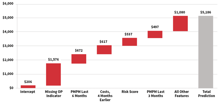
For many modern machine learning algorithms, the relationships between features and predicted values can be complex. The waterfall chart in Figure 2 is a representation of the prediction development for a single member’s IBNR estimate for the most recent month, using a gradient boosting machine. For this member, the model started with a baseline estimate of $206, but this increased by approximately $1,576 as a result of the member having a “missing outpatient claim” (as described earlier). Other features pushed the prediction even higher, including high monthly costs over the past six months and a high risk score. Ultimately, the model predicted an IBNR of $5,186 for this member.
Figure 2: Illustration of Predicted IBNR for Individual Member, Gradient Boosting Machine
Case Study: How Accurate Were Our Models?
To keep our case study simple, our models only predicted claims that were incurred within the three months prior to the valuation date because these months constitute the bulk of the reserve. To evaluate the accuracy of our models, we split the data into two sets: a training set and the testing set. The model was built on the training set while the testing set was withheld for model evaluation and to ensure we weren’t overfitting.
 One of the most important considerations in building a predictive model is which variables to include.
To estimate overall performance, we compared the 10 group-level models for each algorithm to two traditional methods. We then compared the predicted results to the actual IBNR for each method or model, and we calculated the aggregate error across all groups, the average absolute percentage error for each group, and the standard deviation of the percentage error across the groups. These values can be seen in Figure 3. Overall, the gradient boosting decision tree model and the penalized regression model estimated the overall IBNR more accurately and had less variation than the traditional methods. These results suggest that predictive models have the potential to increase the accuracy of reserve estimates. We also found that the member-level predictions from the predictive models generally had a 30 percent to 50 percent correlation with actual results, compared with 20 percent to 30 percent when applying the group-level completion factors to individual members. The member-level correlation statistics are more complicated to aggregate across groups and lag months, so we excluded them from Figure 3.
| Figure 3: Error Metrics for Traditional Methods and Predictive Models | |||
|---|---|---|---|
| Traditional Methods | Aggregate Percentage Error | Average Absolute Percentage Error | Standard Deviation |
| Completion Factor | –3.6% | 42.8% | 72% |
| Projection Method | 8.3% | 43.2% | 47% |
| Predictive Models | |||
| Gradient Boosting Decision Tree |
1.4% | 24.8% | 29% |
| Penalized Regression | –0.1% | 27.1% | 34% |
Considerations
Using predictive analytics for the estimation of IBNR does not mean that actuarial judgment is no longer needed. Beyond the expertise needed in crafting the models themselves, adjustments to IBNR should still be made outside the model or as offsets within the modeling process. These adjustments can include handling new entrants without historical data, claim trends, or any staffing or technological considerations that could impact the backlog of claims.
One of the most important considerations in building a predictive model is which variables to include. Most of the increases in predictive power will not come from more powerful or refined techniques, but rather from more carefully considered and richer input data. For health care, some more obvious variables to consider (when available) are age, gender, plan design and geography of the member. In addition, the temporal nature of IBNR makes the timing of when things happen a key consideration. In designing variables for the model, this should be exploited where possible. For instance, the reporting of less expensive drug claims may precede more expensive inpatient and outpatient claims, or high claims in a prior period may indicate more claims are still outstanding.
Given enough feature creation and enough volume of data, a well-crafted predictive model should be able to discern the most pertinent relationships. As an example of some possible relationships a predictive model might uncover, consider Figure 4. In the first table, we see two variables and their joint impact on the IBNR within our case study (for simplicity we are only considering the amount of unreported claims in the month prior to the valuation date and paid within the next month, which we denote L0). The first variable is the member’s average monthly claims over the past year. The other variable is the “missing inpatient” indicator discussed earlier. Similarly, in the second table in Figure 4, we see another joint relationship that can stratify risk. This time the relationship is between the claims already paid in L0 and the risk score of the member.
| Figure 4: Average IBNR in Lag 0 by Certain Key Features | |||
|---|---|---|---|
| Missing IP Indicator | |||
| Prior Year’s Claims PMPM | Yes | No | |
| $0–$200 | $12,612 | $92 | |
| $200–$400 | $10,152 | $316 | |
| $400–$600 | $15,103 | $391 | |
| $600–$800 | $14,302 | $473 | |
| $800–$1,000 | $17,017 | $530 | |
| $1,000–$10,000,000 | $19,831 | $1,545 | |
| Risk Score | ||||
| Claims Paid in L0 | 0–0.5 | 0.5–1.0 | 1.0–2.0 | 2.0+ |
| $0–$1,000 | $98 | $157 | $217 | $757 |
| $1,000–$2,500 | $1,591 | $1,595 | $2,408 | $5,374 |
| $2,500–$10,000 | $2,170 | $2,492 | $2,029 | $8,361 |
| $10,000–$10,000,000 | $2,231 | $2,934 | $4,954 | $16,225 |
The values shown in each cell represent the average observed IBNR for the most recent incurred month in our training data. As we can see in each chart, these variables are all strongly correlated with IBNR, but together we can stratify the risk more accurately than we can in isolation.
Before involving predictive models in your reserving process, many practical considerations are involved. The first and foremost should be a good understanding of the problem you are hoping to solve. While we mention two possible benefits to using predictive models—increased accuracy of the estimates and more accurate IBNR attribution to individual members within the pool—these benefits may not hold in all cases, depending on the availability of data and the line of business. For a list of potential considerations, see Figure 5.
| Figure 5: Practical Considerations Before Using Predictive Models for IBNR |
|---|
|
One thing to keep in mind is that member-level predictive models need not completely replace traditional actuarial methods to be valuable. In fact, the completion factor method and the projection method described are often blended in practice. IBNR estimates created by member-level predictive models can be similarly blended with any traditional approach. They could also be used not for the results directly, but instead as a way to help understand the drivers of changing IBNR values. Regardless, until enough comfort and sophistication with predictive models is established, the most prudent course of action for any actuary is to do rigorous back-testing and results monitoring before replacing any traditional methods.
Conclusion
Overall, our findings indicate that using predictive models for IBNR estimation is promising. However, our analysis is not definitive; given the volatility in IBNR estimates and the sample size we tested, further research is warranted before concluding that predictive modeling techniques are superior to traditional methods. However, predictive analytics methods need not completely supplant traditional IBNR methods to be valuable. Instead, and more likely, the two approaches can supplement and complement each other. What our analysis does suggest is that this is a productive endeavor to explore. By incorporating predictive models into traditional actuarial methods we might not find the crystal ball that we seek, but with the steady incremental improvements it allows us, we can help advance actuarial practice.
References:
- 1. This differs slightly from incurred but not paid (IBNP) reserves, which would also include claims that have been reported but not yet paid. Throughout this article we use the term IBNR, although the same approach could be applied to IBNP reserves. ↩
- 2. Actuaries often make additional adjustments to this historical cost, including applying an assumed trend and adjusting for seasonality or the number of working days per month. ↩
- 3. James, Gareth, Daniela Witten, Trevor Hastie, and Robert Tibshirani. 2013. An Introduction to Statistical Learning: With Applications in R. New York: Springer. ↩