Making Sense of the Unexpected

Typically, business forecasts are heavily dependent on statistics. While statistics are reliable in many circumstances, such as short-term forecasting, life insurance and pension analysis, statistical forecasting doesn’t capture the dynamics of complex environments because one of its key assumptions—that historical conditions are a valid proxy of future behavior—may not be satisfied. In a dynamic world, medical technology advances, jobs transition from the manufacturing sector to the service sector, safety standards improve, diseases that were considered eradicated (or, like bacteria, permanently fouled) reemerge, robotics influences workloads, lifestyles change and so on.

System dynamics (SD) is a modeling technique designed to describe the behavior of systems over time. Interconnections among components, especially those that lead to feedback (whereby an action eventually leads to more changes in the same lever), are a key feature of the method. Time delays also are properly represented in the models. SD is a powerful supplement to statistical forecasting, as each technique is well-suited to tackle problems with different characteristics.

To illustrate: As medical technology improves, people live longer, so population increases. As population grows, the demand for medical technology is fueled, which creates more revenue to further improve medical technology. This is called reinforcing feedback, because the original action (improvement in medical technology) is eventually increased, that is to say, reinforced.¹

In another example, as reinsurers compete for new and renewal business, they reduce premium rates. Eventually, premium collected won’t be enough to cover losses and make a profit. The natural reaction is to raise prices until business becomes profitable again, a process that can take years. But once this goal is achieved, reinsurers start competing to gain market share. The process repeats itself as reinsurers try to capture market share and be profitable. In the lexicon of SD, reinsurers try to keep the system near its goal through a balancing feedback mechanism.

An SD model mirrors the workings of reality as much as is reasonable, but purposefully leaves out irrelevant details that complicate the model without improving it and, frequently, make it less robust. For instance, if we are modeling the population of a country or region, there will be accumulations of people (called stocks and represented with a box in Figure 3) in different cohorts. Each cohort has its own death and migration rates, which cause these stocks to change (through flows, represented with pipes with valves on them in Figure 3). What is happening in the world—war, disease, medical technology, economic condition and so on—can affect these rates. Furthermore, these influences are not stationary and can themselves be influenced by the population.

Observations About Correlation and Probabilities

The tools employed to model many (certainly not all) the phenomena that take place in business trend the past to predict the future, perhaps with some indication of the range of uncertainty. Because these techniques (almost always a form of regression) are not designed for long-term predictions, nor necessarily to understand how variables interact, they can misrepresent causation and correlation. To appreciate the problem, consider sample populations of college students in their senior year from 1976 to 2015. Average medical costs and the average concentration of certain amino acids are recorded and plotted in Figure 1 where, after suitable scaling adjustments, the left y-axis represents average medical cost and the right y-axis represents average amino acid concentration.

The following conclusions are plausible:

• The amino acid concentration has increased over time.
• Lower medical costs are associated with moderate amino acid concentration.
• Patients should take a drug that brings the amino acid concentration to optimal levels to reduce both morbidity and medical expenses.

In this hypothetical illustration, we have attributed causation where it doesn’t exist. It turns out that body mass index (BMI) determines amino acid concentration and medical cost. Accordingly, risk-adjusting medical costs based on amino acid concentration is clearly a mistake, and the use of drugs to bring the concentration of the amino acid to “optimal” levels is not only ineffective but perhaps harmful. Yet, the correlation coefficient suggests otherwise.

In many instances where regression and its variants are used, it is entirely feasible to determine causation. But with big data and increased computing power, the odds of making erroneous attributions are magnified. Moreover, since it is possible to be selective in the collection of data, different conclusions can be reached, sometimes unintentionally due to the overwhelming amount of information, sometimes in response to a modeler’s bias. With too much information (not all of which is useful), it can be impractical to review the logic of models that capture a great amount of detail. Finally, it is always possible to over-calibrate and “predict” the past with an accuracy that won’t be carried forward in the future.

What about using probabilistic models to estimate outcomes such as expected medical costs without a good grasp of the causal relationships? Here the problem is often associated with the difficulty in understanding, from time series or similar data, how variables interact, and with simplifying assumptions that, however necessary, could be erroneous, such as probabilistic independence. To illustrate: Whereas it is true that the behavior of water molecules is statistically identical, the behavior of people is not. There is no uniformity of thought and feeling; human behavior has elements of randomness and irrationality; genetic makeup plays a role; recovery rates can be individual-based; the environment changes; and so on.

How do we know whether or not a model is reliable? The following criteria come to mind:

• Model structure. Is the model consistent with the facts? Does the model reflect our knowledge of how the real world operates? Does the model capture the key elements of reality and ignore those that are superfluous for our purposes?
• Model behavior. Are simulations consistent with observations?
• Learning. It is possible to conduct “experiments” with a simulator to understand how the system works and to test hypotheses. Have users gained insights about the system structure or learned something new about the behavior of the system?

Two case studies can illustrate the use of SD with real-world problems.²

Case Study 1: Firm Growth

You have invested for years in your company, Galaxy Consulting, which has finally taken off. You believe that the best way to motivate high performers and to ensure they remain committed to Galaxy is to make them corporate owners. For partners, performance determines the number of client engagements, which in turn influences compensation and work load. Since the number of partners is directly related to growth, you are interested in determining the most appropriate promoting and hiring policies. Keep in mind that, on the one hand, you want Galaxy to attain economies of scale and, on the other, maintain the reputation of reliability that is Galaxy’s most important asset—losing it would not only compromise growth but also survival. To determine the optimal growth strategy, you and your team develop the causal diagram in Figure 2.

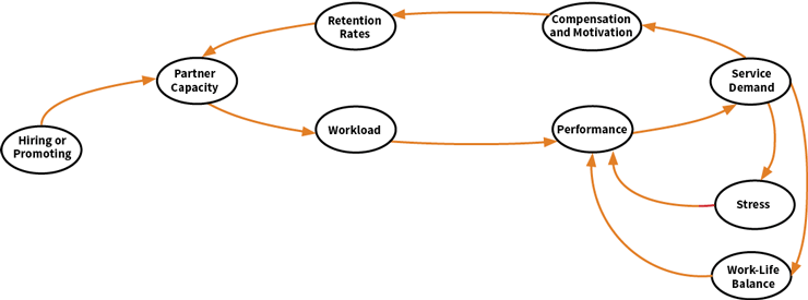
As you promote or hire, the pool of partners grows, easing workload per partner and improving performance. Client satisfaction generates demand, which in turn motivates and rewards partners financially. The result is the intended high retention rates. However, as demand for services grows, work-life balance suffers and the corrosive effects of stress become discernible. This takes a toll on performance, demand diminishes, motivation is reduced and compensation is curtailed. Some of the people in whom you have invested heavily leave Galaxy, putting more pressure on those who stay. You want to avoid this situation at any cost. What can you do? The pipeline of potential partners is limited (your company is still small) and you know that new executives need time to adapt to Galaxy’s culture, learn about your services and earn your trust. Clearly, there is a point beyond which growth can be dangerous, but where is it?

To answer this question, you must quantify the relationships between variables. For example, research may indicate that a 10 percent increase in compensation improves retention rates by 5 percent; a weekly reduction of 10 hours of family time increases errors by 2 percent; when reported stress jumps 10 percent, peer-review time grows 20 percent; and so on. You will try to quantify relationships using functions that are as detailed as possible, but only if they have explanatory power.

Modelers spend most of their time developing causal maps and quantifying relationships between variables. The next case study illustrates the latter, with an example that is well-known to actuaries.

Case Study 2: Social Security

Imagine you are analyzing different policies to ensure the solvency of the Social Security program in the face of a greater ratio of retired people to working people combined with increasingly lower average salaries. To do this effectively, you will need to age the population and include proper accounting for both monies collected and monies due.

Figure 3 shows a population model with separate cohorts for ages 0–14, 15–29, 30–44, 45–64, and 65 and up (these are the boxes). People from ages 15–44 reproduce to create children who are born (far left). On the far right, people die of old age. The variable “time as senior citizen” specifies the number of years someone survives—on average—after reaching age 65. In between, people age through their lives to however long they live.

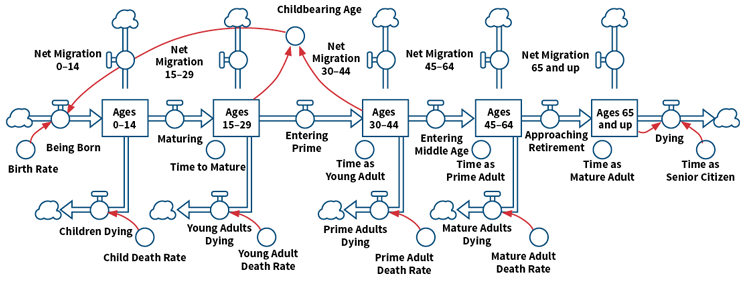
Note that the last category is labeled “Ages 65 and up.” While the model is initially parameterized this way, this stock can easily be changed to contain retired people by adjusting the parameter “time as mature adult.” In this way, different policies related to retirement age can be tested. In addition, as medical technology improves, the parameter “time as senior citizen” can be extended. The birth rate, migration rates and mortality rates in each age group also can be varied to see the effects under different scenarios.

Running the model with census bureau parameters shows the population growing over 50 years (see Figure 4). Note the retired population (Ages 65 and up, dashed orange line) is growing at a healthy rate. While it is not evident from this graph, the working population (Ages 15–64, dashed red line) is growing at a slower rate. This is clearer in Figure 5 (solid blue line), which shows the ratio of retired people to working people. From 2012 to 2052, this ratio grows 70 percent.

The implications of these findings are startling and by now well-documented. Since Social Security benefits are cash transfers from the working population to retirees, the burden on the working population almost doubles in 50 years. If you consider that the average salary is falling over the same period, the burden easily doubles. Finally, if you consider extended life expectancies, five years in this case, the situation becomes even worse (Figure 5, dashed orange line).

This model, as it stands, does not include the accounting for monies collected and due. Nor does it simulate the improvements in medical technology that can extend life expectancy. While these and other variables can be added, the model provides useful insights even without them. For example, if the retirement age is increased from 65 to 70 over 50 years, it is possible to stabilize and reverse the ratio of retired to working people (Figure 6, dashed red curve).

Conclusion

Perhaps the greatest strength of SD is its emphasis on understanding how complex systems work, what matters, what does not and how levers interact. If you understand the problem, you can model it. If you model it, but simulations or predictions are incorrect, then your understanding is deficient. When this happens, as you improve the model, your knowledge of the system is enhanced and you gain strategic insights.

References:

- 1.For a description of the elements of system dynamics, see: Sanchez-Fuentes, Carlos. “System Dynamics: Building a Better Model.” Contingencies. Sep/Oct 2011, 36–41. ↩
- 2. For additional examples, see: Gottfried, Dennis, and Carlos Sanchez-Fuentes. “Modeling Obesity.” Contingencies. Nov/Dec 2012, 38–45, and Srijariya, Witsanuchai, Arthorn Riewpaiboon and Usa Chaikledkaew. “System Dynamic Modeling: An Alternative Method for Budgeting.” Value in Health 11 (2008). ↩