
Costly Trends
Measuring claim cost movement in volatile markets
December 2018/January 2019Statements of fact and opinions expressed herein are those of the individual author(s) and are not necessarily those of the Society of Actuaries or the respective authors’ employers.
The measurement of health care cost growth is a crucial element in pricing health insurance products. Trend rates are used to project a company’s claims experience into future time periods. While projecting trends was never an easy exercise, the implementation of the Affordable Care Act (ACA) resulted in material changes to the health insurance market that made analyzing trend even tougher. The Office of the Assistant Secretary for Planning and Evaluation (ASPE) estimated that premiums for individual market coverage increased 105 percent from 2013 to 2017 after the passage of the ACA.1
These substantial increases result from a wide range of underlying factors, including ACA provisions and recent federal administrative actions. For example, new regulations and laws regarding association health plans,2 short-term medical plans3 and the nonenforcement of the individual mandate penalty4 will likely cause individual market premiums to increase further and make it more difficult to isolate trend from other market changes when reviewing historical experience.
The increase of medical costs historically has been the single most important factor that causes health insurance rates to rise. Three major components comprise medical trend:
- Increases in the cost of a given medical service or procedure
- Increases in the use of medical services and procedures
- The intensity or mix of services provided
While prospective insights on the impact of the changes in the individual market are important in developing actuarial projections, the medical trend estimate based on historical data is still considered the most important component. Considerable analysis must be performed on a retrospective basis to validate prior projections and to assess emerging results.
Traditional Trend Methods
Trend analysis requires much thought and is not just a number-crunching exercise. Medical trend estimation is a complicated process, and a variety of methods can be used to analyze claims trends. Whatever methods are selected, it is important that an actuary fully understand the methods used, including their strengths and their weaknesses. Failure to analyze the trend study properly could result in trends that are less predictive.
Figure 1 shows the data used for our analysis. The 48 months of data are representative of data from a carrier that sells qualified health plans (QHPs) in the ACA individual market. A company that has a large, statistically credible block of business may analyze trend at the component level—for instance, unit cost and utilization or trends by service category. For simplicity, we analyzed the trends at the aggregate level.
| Figure 1: Historical Claims and Membership | |||||||
|---|---|---|---|---|---|---|---|
| Month | Members | Allowed Costs | Allowed PMPM | Month | Members | Allowed Costs | Allowed PMPM |
| 1/1/14 | 37,641 | $10,464,115 | $278.00 | 1/1/16 | 172,671 | $66,478,435 | $385.00 |
| 2/1/14 | 37,528 | $10,840,522 | $288.87 | 2/1/16 | 172,326 | $59,571,585 | $345.69 |
| 3/1/14 | 37,453 | $10,953,444 | $292.46 | 3/1/16 | 172,154 | $62,161,654 | $361.08 |
| 4/1/14 | 37,340 | $11,668,617 | $312.49 | 4/1/16 | 171,809 | $66,478,435 | $386.93 |
| 5/1/14 | 37,228 | $10,464,115 | $281.08 | 5/1/16 | 171,637 | $64,233,709 | $374.24 |
| 6/1/14 | 37,154 | $10,388,833 | $279.62 | 6/1/16 | 171,123 | $61,816,311 | $361.24 |
| 7/1/14 | 37,042 | $11,819,180 | $319.07 | 7/1/16 | 170,609 | $65,097,065 | $381.56 |
| 8/1/14 | 37,005 | $11,104,007 | $300.06 | 8/1/16 | 170,097 | $65,615,079 | $385.75 |
| 9/1/14 | 36,894 | $10,539,396 | $285.66 | 9/1/16 | 169,757 | $60,434,941 | $356.01 |
| 10/1/14 | 36,784 | $12,195,587 | $331.55 | 10/1/16 | 169,587 | $60,952,955 | $359.42 |
| 11/1/14 | 36,710 | $11,292,210 | $307.60 | 11/1/16 | 169,248 | $59,571,585 | $351.98 |
| 12/1/14 | 36,637 | $11,367,491 | $310.28 | 12/1/16 | 168,740 | $60,952,955 | $361.22 |
| 1/1/15 | 41,823 | $14,052,528 | $336.00 | 1/1/17 | 177,486 | $72,946,795 | $411.00 |
| 2/1/15 | 41,739 | $15,307,218 | $366.73 | 2/1/17 | 177,309 | $74,544,170 | $420.42 |
| 3/1/15 | 41,698 | $13,676,121 | $327.98 | 3/1/17 | 176,954 | $72,236,851 | $408.22 |
| 4/1/15 | 41,573 | $15,432,687 | $371.22 | 4/1/17 | 176,777 | $66,912,267 | $378.51 |
| 5/1/15 | 41,448 | $15,474,510 | $373.35 | 5/1/17 | 176,247 | $73,124,281 | $414.90 |
| 6/1/15 | 41,406 | $14,428,935 | $348.47 | 6/1/17 | 176,070 | $74,366,684 | $422.37 |
| 7/1/15 | 41,324 | $13,968,882 | $338.04 | 7/1/17 | 175,718 | $68,687,128 | $390.89 |
| 8/1/15 | 41,200 | $15,599,979 | $378.64 | 8/1/17 | 175,543 | $70,107,017 | $399.37 |
| 9/1/15 | 41,117 | $13,717,944 | $333.63 | 9/1/17 | 175,367 | $72,236,851 | $411.92 |
| 10/1/15 | 41,035 | $13,968,882 | $340.41 | 10/1/17 | 175,016 | $74,189,198 | $423.90 |
| 11/1/15 | 40,912 | $15,390,864 | $376.20 | 11/1/17 | 174,666 | $73,301,768 | $419.67 |
| 12/1/15 | 40,871 | $14,303,466 | $349.97 | 12/1/17 | 174,142 | $74,721,657 | $429.08 |
Calendar year data from 2014–2016 was used as the experience period to project trend through the end of 2017. The actual 2017 data was used to analyze the results of the methods used.
The trend analysis is focused on allowed costs.5 This approach removes the impact of consumer cost-sharing. Increases in claim costs can be severely leveraged when deductibles do not increase with trend each year.
Root Mean Square Error (RMSE)
The root mean square error (RMSE) can be used to evaluate the models tested. A lower RMSE means the model is a better fit. However, caution should be used when comparing results across different time periods (e.g., 24 months versus 36 months of data). For example, if the data from month 25 to month 36 is more volatile from month to month, this will increase the RMSE, but it does not necessarily mean that the methods using 36 months of data are less predictive.
Determining Which Method to Use
Linear regression is a well-known method that is used in prediction and forecasting. In linear regression, it is assumed there is a linear relationship between the observed and estimated values.
Another common method is exponential regression. This method assumes the linear relationship exists between the transformed response and explanatory variables (instead of the original variables). Exponential regression is often preferable in medical trend analysis, as it assumes the increasing rate over the interval is a constant.
When the data is stable and the trend factor is small to moderate in magnitude (e.g., 10 to 20 percent), estimation by linear regression and exponential regression often produce similar results over a short period, with linear regression producing lower trends than exponential regression.
Besides determining the method, another decision that needs to be made is how much of the historical data should be used. Our analysis includes methods that use both 24 months and 36 months of historical data.
Seasonality is a common phenomenon in monthly health insurance data. Many actuaries prefer using a rolling 12-month method to address seasonality. Therefore, we also used a rolling 12-month method over a 24-month period to address any underlying seasonality patterns.
Adjusting for Demographics and Benefit Changes
Actuaries understand that a block’s underlying population can shift from year to year. Before the ACA, actuaries primarily adjusted the underlying data for lurking variables such as geographic mix and the age-gender (AG) distribution. However, the ACA has created markets that are often more volatile year over year.
To account for demographic differences by calendar year, the data was normalized by the average AG factor each month. By analyzing allowed claims, the impact of varying cost-sharing is mitigated. However, it is still important to normalize for changes in induced utilization6 if the benefit levels have changed during the experience period. Figure 2 summarizes the AG and induced utilization factors used. For each month, the actual allowed claims were divided by monthly AG and induced utilization factors.7
| Figure 2: Age-Gender and Induced Utilization | ||
|---|---|---|
| Year | Age-Gender | Induced Utilization |
| 2014 | 1.504 | 1.071 |
| 2015 | 1.521 | 1.072 |
| 2016 | 1.477 | 1.032 |
| 2017 | 1.498 | 1.035 |
Figure 3 compares the results of the base projection methods for projecting allowed costs into 2017. The solid lines are the predicted best estimates while the dotted lines are the 95 percent confidence interval for a given method. For display purposes, only the 2016 experience period is illustrated.
Figure 3: Linear and Exponential Regression—Projected PMPM Costs
Click Image to Enlarge
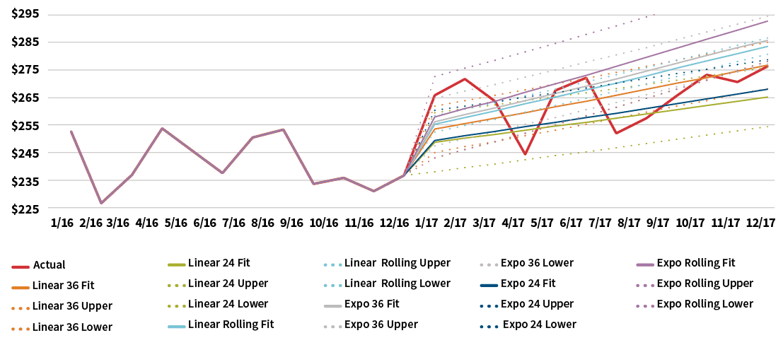
One observation is that the 24-month regression produces significantly lower per-member per-month (PMPM) costs than the 36-month methods. The projected differences resulting from the different time periods used obviously are a consideration when selecting a final trend estimate.
Figure 4 illustrates the trend estimates based on each of the base regression methods used. Each trend estimate is based on dividing the projected 12-month rolling PMPM cost ending Dec. 31, 2017, by the 12-month rolling PMPM cost ending Dec. 31, 2016. Not surprisingly, the rolling PMPM methods have the lowest error measures since they are based on smoothed and aggregated data. The 24-month exponential and linear methods have different trend estimates even though they have similar error measures. This highlights that the “best fit” is not always the easy answer, and there are a lot of considerations in trend estimation.
| Figure 4: Regression Results—AG and Induced Utilization Adjusted | ||
|---|---|---|
| Method | Trend Estimate | PMPM RMSE |
| Linear regression, 24 months | 7.2% | $12.14 |
| Exponential regression, 24 months | 8.1% | $12.19 |
| Linear regression, 36 months | 10.1% | $11.99 |
| Exponential regression, 36 months | 12.7% | $14.63 |
| Linear regression, 12-month rolling | 12.2% | $3.34 |
| Exponential regression, 12-month rolling | 14.9% | $3.82 |
| Adjusted actual | 9.9%8 | |
Adjusting for Morbidity
In Figure 3, some of the base methods appeared to produce reasonable trend estimates. However, as mentioned previously, there was a dramatic increase in membership from 2015 to 2016 that should be analyzed for any significant morbidity shifts. Therefore, the next step in the analysis was to account for any underlying morbidity differences by calendar year. This was accomplished by normalizing the data by the plan level risk score (PLRS). The ACA-defined PLRS accounts for age, so the previously used AG factors were replaced in this step.
Before the PLRS can be used to normalize the historical claims, an adjustment needs to be made to account for morbidity changes in the underlying risk adjustment model that calculated the PLRS values. Since the creation of the risk-adjustment program, the Centers for Medicare & Medicaid Services (CMS) has annually enhanced the underlying models. These enhancements were undertaken to use updated data and information to better predict the risk scores of the covered populations.
This is one adjustment to the data set that may not have been intuitively considered from the beginning; however, it could have a substantive impact on projecting future trends for a carrier. If the methods used to calculate PLRS have been modified during the experience period, then the historical PLRSs must be adjusted to create better projection models.
Figure 5 illustrates the PLRS factors used to further normalize the allowed costs. For each month, the actual allowed claims were divided by the adjusted PLRS. This adjusts the claims so that each exposure period can be compared without concern for morbidity changes in the population.
| Figure 5: Adjusted PLRS | ||
|---|---|---|
| Year | PLRS | |
| 2014 | 0.941 | |
| 2015 | 0.993 | |
| 2016 | 1.052 | |
| 2017 | 1.125 | |
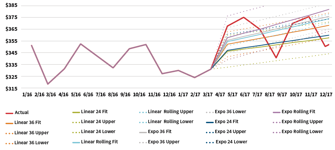
Figure 6 graphically compares the results of the base regression methods after normalizing the data for population morbidity, while Figure 7 illustrates the resulting trend estimates based on the projected PMPM costs in Figure 6.
Figure 6: PLRS Adjusted Regression—Projected PMPM Costs
Click Image to Enlarge
| Figure 7: Trend Analysis—PLRS Adjusted | ||
|---|---|---|
| Method | Trend Estimate | PMPM RMSE |
| Linear regression, 24 months | 1.3% | $15.10 |
| Exponential regression, 24 months | 1.3% | $15.10 |
| Linear regression, 36 months | 5.7% | $17.03 |
| Exponential regression, 36 months | 6.4% | $17.26 |
| Linear regression, 12-month rolling | 5.9% | $4.83 |
| Exponential regression, 12-month rolling | 6.5% | $5.03 |
| Adjusted actual | 4.2%9 | |
After this round of normalization, the range of results have narrowed and the most significant variation is between the methods that use 24 and 36 months of data. This variation between the historical periods should be considered in light of the material membership jump from 2015 to 2016. Alternatively, an actuary could analyze the 24 months of data from 2014 to 2015 to remove the impact of the jump in membership.
Alternative Trend Analysis Methods
The primary purpose of medical trend analysis is to forecast future medical costs. While a few of the common regression methods appear to be reasonable fits for the data set, there are a variety of methods that should be considered. While additional methods may or may not produce better estimates, the evaluation of additional methods allows the actuary to see the whole “story” the data set is telling.
While we will not describe each specific method used, here is a summary of two general approaches— autoregressive (AR) models and moving average (MA) models—that should be considered in a trend study in addition to linear and exponential regression methods.
Autoregressive (AR) Models
Medical costs are clear examples of time series data. Therefore, traditional time series analysis can be useful in forecasting future claim levels. In an autoregression model, the forecasted value is based on a linear combination of past values of the variable. That is, the goal is to isolate patterns in the past data.
Autoregressive models can be important in analyzing health care data where seasonal utilization and underlying lurking variables—for example, morbidity—can muddle the estimation of trend.
Mathematically, unlike regression methods, time series methods assume that estimation errors are correlated for some time period. Intuitively this makes sense since the medical cost of a period is likely to have some correlation with former time periods.
Moving Average (MA) Models
Rather than using past values of the forecast variable in a regression, a moving average model uses past forecast errors in a regression-like model. Each projected value can be thought of as a weighted moving average of recent forecast errors.
Figure 8 compares the results of the additional methods using 24 months of historical data.
Figure 8: 24-Month Time Series Methods—Projected PMPM Costs
Click Image to Enlarge
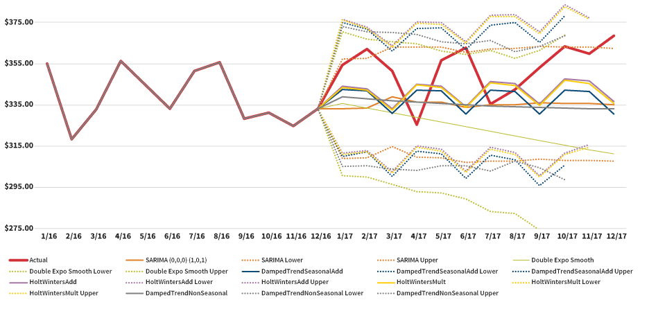
Figure 9 compares the results of the additional methods using 36 months of historical data.
Figure 9: 36-Month Time Series Methods—Projected PMPM Costs
Click Image to Enlarge

Figure 10 illustrates the resulting trend estimates based on all the methods used in the trend study.
| Figure 10: Trend Summary—All Methods | ||
|---|---|---|
| Method | Trend Estimate | Root Mean Squared Error |
| Linear regression, 24 months | 1.3% | $15.10 |
| Exponential regression, 24 months | 1.3% | $15.10 |
| Linear regression, 36 months | 5.7% | $17.03 |
| Exponential regression, 36 months | 6.4% | $17.26 |
| Linear regression, 12-month rolling | 5.9% | $4.83 |
| Exponential regression, 12-month rolling | 6.5% | $5.03 |
| SARIMA (0,0,0) (0,0,1) 24 months | –1.0% | $12.26 |
| Double exponential regression smoothing, 24 months | –4.5% | $17.77 |
| Damped trend seasonal additive, 24 months | –0.2% | $16.49 |
| Damped trend seasonal multiplicative, 24 months | –0.2% | $16.53 |
| Holt winters additive, 24 months | 0.9% | $16.57 |
| Holt winters multiplicative, 24 months | 0.7% | $16.60 |
| Damped trend non-seasonal, 24 months | –1.0% | $17.33 |
| SARIMA (1,1,1) (0,0,2) 36 months | –3.0% | $14.47 |
| Double exponential regression smoothing, 36 months | –3.7% | $17.82 |
| Damped trend seasonal additive, 36 months | –2.2% | $18.03 |
| Damped trend seasonal multiplicative, 36 months | –2.1% | $18.08 |
| Holt winters additive, 36 months | –3.3% | $18.40 |
| Holt winters multiplicative,36 months | –3.2% | $18.51 |
| Damped trend non-seasonal, 36 months | –2.1% | $17.46 |
| Adjusted actual | 4.2% | |
Interestingly, the time series methods presented in Figure 10 predict PMPM costs that are lower than the actual results. The initial reaction might be to infer that these methods are not very informative since they may not be as predictive as the other methods; however, we believe these methods do help in setting the trend. These methods tell us there may be some downward pressure in the data set that may not be easily recognizable by using traditional regression methods.
As we saw in the results from the regression methods, those estimates were generally higher than the actual results. By using the times series results, an actuary may feel more comfortable setting a trend lower than what the regression methods project.
Conclusion
Every actuarial projection is an attempt to predict and model what will happen in the future. Every actuary knows that no projection can be 100 percent correct; however, an actuary should always strive to understand all variables that may affect a projection.
Additionally, this discussion was not designed to promote the use of one trend model over another. There are a lot of methods that we did not have the opportunity to discuss such as Monte Carlo simulation methods. An actuary should use all techniques available to him or her, not just the standard methods that have always been used.
If the analysis of more underlying variables and the use of new methods can produce a better picture of what might happen in the future, the actuary can gain a greater understanding of all of the factors that can impact future financial results. The actuary can use the original assumptions and projections to monitor actual results and to enhance the trend process in future time periods.
References:
- 1. U.S. Department of Health and Human Services Office of the Assistant Secretary for Planning and Evaluation. Individual Market Premium Changes: 2013–2017. U.S. Department of Health and Human Services: ASPE Data Point, May 23, 2017, (accessed September 8, 2018). ↩
- 2. Employee Benefits Security Administration, Department of Labor. Definition of ‘‘Employer’’ Under Section 3(5) of ERISA—Association Health Plans. Federal Register 83, no. 120:28912, (accessed September 10, 2018). ↩
- 3. Internal Revenue Service, Department of the Treasury; Employee Benefits Security Administration, Department of Labor; Centers for Medicare & Medicaid Services, Department of Health and Human Services. Short-Term, Limited-Duration Insurance. Federal Register 83, no. 35:7437, (accessed September 10, 2018). ↩
- 4. United States Congress. Public Law 115–97: Individual Tax Reform and Alternative Minimum Tax. December 22, 2017, (accessed September 10, 2018). ↩
- 5. Allowed costs are the maximum amount on which payment is based for covered health care services. These are the costs before consumer cost-sharing is applied. ↩
- 6. Induced utilization is defined as the additional demand for services created by an increased level of coverage regardless of health status. ↩
- 7. Additional normalization factors may be necessary depending on the underlying data. Examples include network, geography and changes to company programs. ↩
- 8. The actual PMPM changes from 2016 to 2017 include changes in demographics, benefits levels and morbidity. The actual results for 2017 are adjusted using the same methods as the historical experience. ↩
- 9. Ibid. ↩
Copyright © 2018 by the Society of Actuaries, Chicago, Illinois.