How Could Environmental Risk Modeling Help Shape Actuarial Education?

Photo: iStock.com/piyaset

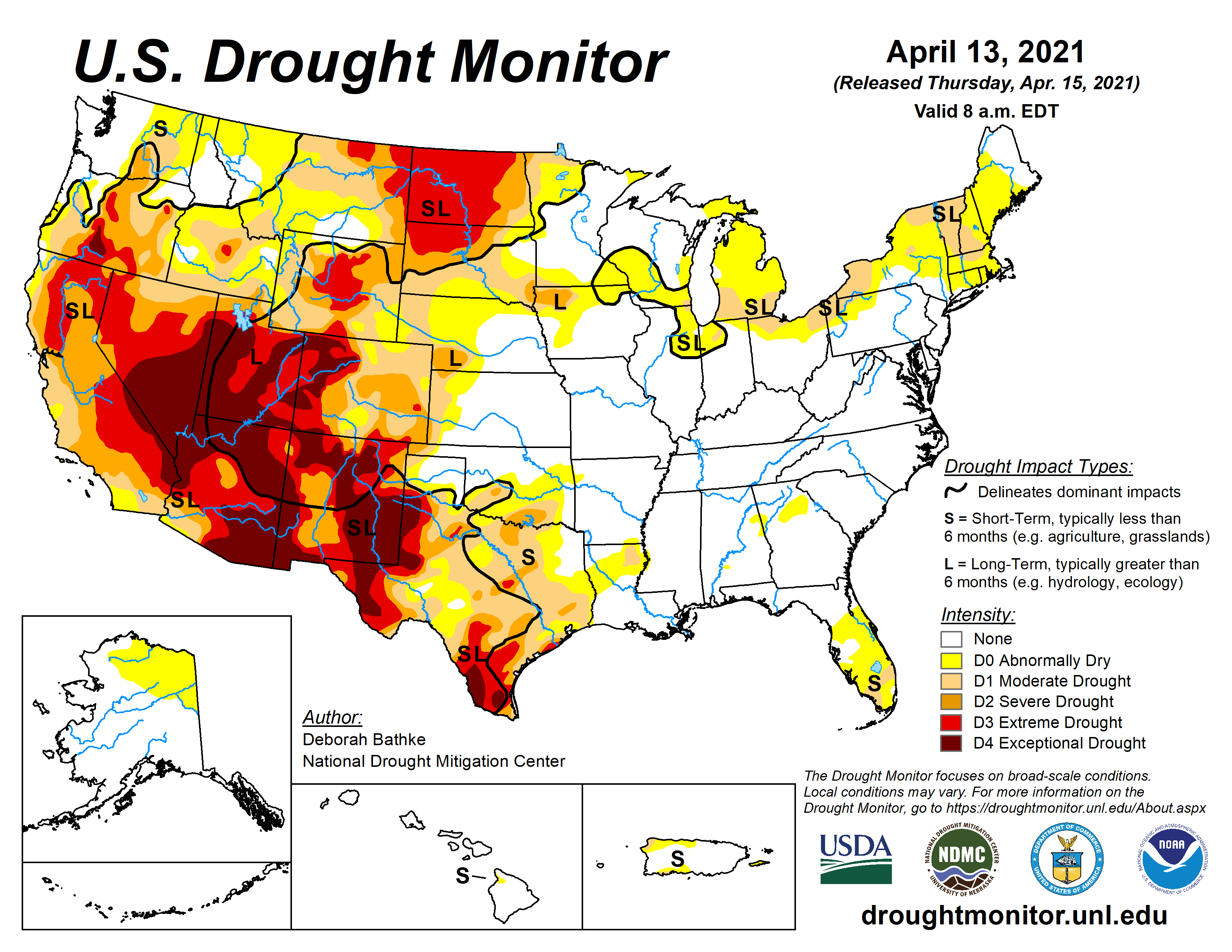
At the time of this writing (April 2021), much of the Western United States was experiencing either extreme or exceptional drought (see Figure 1). The U.S. Drought Monitor (USDM)—the nation’s foremost data product on drought conditions—defines extreme drought as major crop and pasture losses with widespread water shortages or restrictions.^1,2 Taking it a step further, exceptional drought means widespread crop and pasture losses and shortages of water in reservoirs, streams and wells creating water emergencies. Both mean a role for insurers and actuaries.

Articles on the accumulating negative consequences of drought regularly feature the USDM. The Economist recently reported: “Because drought is a perennial problem in the West, adaptation has become a way of life. Some farmers in Colorado and the northwest are experimenting with farming without irrigation. Colorado’s proposed COVID-19 stimulus plan includes up to $55 million to fight drought and fire.”³ The Washington Post has sounded an alarm for the upcoming fire season in California, recently publishing an article entitled “Drought-plagued California and Western U.S. May See Another Devastating Fire Season.”⁴

Drought risk management is on the minds of many, and insurance is part of that management. It makes sense that a high-quality data product on drought may contain useful information for modeling property and crop losses resulting from droughts. When coupled with projections from the National Oceanic and Atmospheric Administration’s (NOAA’s) Climate Prediction Center, this data could help inform planning and risk management. Therefore, imagine a hypothetical actuary tasked with an analysis focused on crop losses. What skills would they need to explore fully the benefits of using the USDM?

Digging into the Data

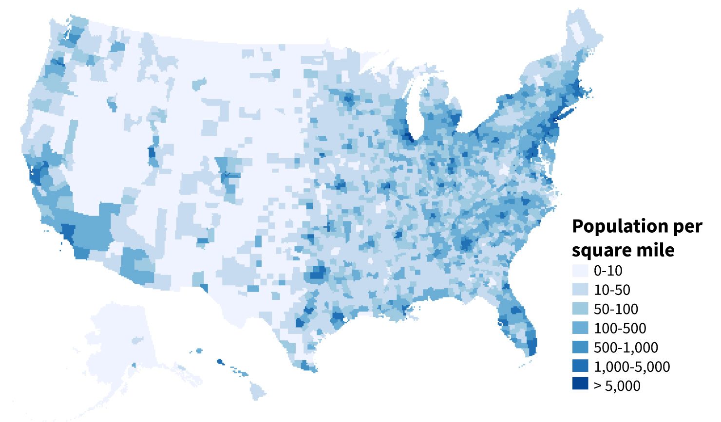
Let us begin with the data. The USDM would be one data set among many. The response variable would probably be a loss measure. Perhaps the hypothetical actuary would start with the Spatial Hazard Events and Losses Database for the United States (SHELDUS),⁵ a county-level database on hazards and direct losses. A quick glance shows dramatically different crop losses across the United States, but this is partly due to varying exposures. Normalizing by population makes sense, but it requires county-level population data from the U.S. Census Bureau (see Figure 2). Perhaps normalizing by acreage under cultivation makes more sense, and the actuary includes county-level data from the U.S. Department of Agriculture.

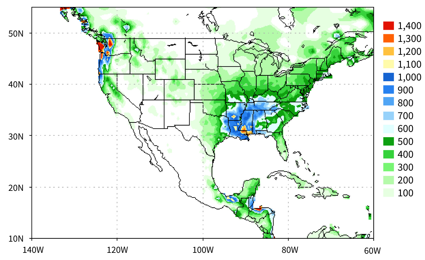
Of course, there are other known drivers of crop losses, and these would need to go into the model as well. Maybe controlling for soil type is important, with remotely sensed data from NASA’s Land Data Assimilation System. Other climate data, such as accumulated precipitation, can help, and the actuary turns to NOAA’s Climate Prediction Center and its various gridded data products (see Figure 3).

In actuarial analyses, garbage in means garbage out. The actuary must strive to find quality data and not miss important disclaimers. Before any modeling begins, they read data descriptions and companion papers written by demographers, meteorologists, data scientists and soil scientists. Furthermore, these papers describe a dizzying array of data types.

• The USDM is a shapefile, which stores geographic information for features as points, lines and polygons, and ties attributes to these features (refer back to Figure 1).
• Areal data describes aggregated measurements over regions with a neighborhood structure, and examples include the county-level data from SHELDUS, the U.S. Census Bureau and the U.S. Department of Agriculture (refer back to Figure 2).
• Remotely sensed data products and many climate variables are stored as gridded rasters (refer back to Figure 3).

Manipulating these various data structures requires knowledge of geographic information system (GIS) software. Our hypothetical actuary will need to merge the data to support an actuarial analysis. Shapefiles of the USDM intersect with counties to attribute a drought level to each county and month. Rasters intersect with county borders to identify which data goes where in the merged data set. At some point, the actuary discovers the number and borders of U.S. counties have changed since 1960. Even an experienced programmer may need to reach for a scientific textbook such as Geocomputation in R.

Despite these challenges, imagine the actuary succeeds to produce a clean data set. Next, they move to the modeling phase. Location and time probably index each observation; that is, the exposure units are likely spatial and temporal. Waldo Tobler’s so-called first law of geography is “everything is related to everything else, but near things are more related than distant things.”⁶ In our setting, near can mean physically close in space or temporally close in time, and related means statistical dependence.

Data for environmental actuarial analyses, it turns out, is unavoidably spatio-temporal. In other words, observations are not independent. The actuary bids farewell to the standard implementations of linear models and generalized linear models; they instead turn to random effects, mixed-effects models, time series and spatial statistics.

The Necessary Skill Set

I began this article with the premise that a data product on drought is likely to have value when modeling insurance losses caused by this environmental hazard. This led me to enumerate what an analyst would need: basic environmental science literacy, skill with geocomputational data science and advanced statistical models. Keep in mind that drought is only one example. I could easily consider floods or hurricanes, and a similar story calling for a similar set of skills would unfold each time.

So, which of these skills do actuaries have?

Overall, actuaries have very few of these skills. The standard actuarial exams omit most of these topics and only touch the surface of the remainder. There is a lot of material to cover, and trade-offs are unavoidable. However, I posit that this hypothetical actuary could learn all of these things. Perhaps not to the level of expert, but certainly to a basic proficiency.

The exam process leads every actuary to encounter some novel topics (e.g., accounting, regulation, rate making, regression trees, etc.). Actuaries are already in the business of self-study, and they have demonstrated success in this regard.

Which skills could and should they learn?

Should the actuary learn these skills? Or could the IT department handle the database construction instead by hiring programmers to work with shapefiles, rasters and areal data? Are consultants available to give advice on data sources drawn from meteorology and geology? What about hiring statisticians to fit spatio-temporal models and give crisp, interpretable statements to inform business decisions?

These are fair questions, which I answer with another: Even if a company sourced each step as described, wouldn’t the actuary still be responsible for business decisions based on the output from the analysis? Actuaries, not IT departments, sign statements of actuarial opinion. These statements mean something because of the high professional standards of actuaries. Every actuary knows that certifying the recommendation from an analysis means certifying the entire process—from raw data to final output—and this is true even when the analysis involves spatio-temporal environmental data.

Two Groups of Actuaries

To conclude, let’s widen the focus, turn to all actuaries and divide them into two groups:

1. The first group, which probably describes most actuaries, contains those who do not encounter environmental risks much in their professional duties. While not entirely disconnected from climate risk, the meteorological, spatial and temporal considerations discussed in this article do not relate strongly to this group’s actuarial practice, and its members are unlikely to conduct an analysis similar to what has been described.
2. The second group more closely connects to environmental risk. Perhaps its members work in property insurance or support reinsurance and are forced to think about extreme weather events. Perhaps its members keep hearing at conferences how climate risk has implications for their work. This group is admittedly smaller, but it is not trivially small.

How should environmental risk inform actuarial education for each group? First, both groups should learn mixed-effects models. These models add one or more random effects to familiar fixed effects. They are widely used for observations that fall short of statistical independence in some meaningful way, and as such, they are a gateway to modeling exposures that do not satisfy the “independent and identically distributed” assumption of textbooks. Actuaries already contend with mathematical models just as complex—computational power has grown tremendously in recent years and available software can fit these models in a reasonable amount of time. Upon reflection, I suspect most actuaries can find examples from their practice areas where these models could give greater insight.

Second, both groups of actuaries should learn to merge multiple data sets within a reproducible programming environment. By reproducible, I mean a scripted computer program that the author passes along to a colleague who can re-run it and produce an identical database. Most data sets needed to explore environmental risks simply do not exist right now—they must be built from smaller data sets. This condition is not unique to environmental work, as it holds true for all practice areas in actuarial science. Actuaries cannot merely pull subsets from existing company databases. They must be able to envision data sets not currently stored on company servers. They will need basic programming and database proficiency to play a meaningful role in the construction of these new data sets.

Finally, I concede that many actuaries in the first group probably do not need to learn about shapefiles, spatial statistics or environmental science. There are more pressing priorities for their professional development. However, the second group surely contains intrepid actuaries who have both the will and the need to model environmental risks more fully. Their employers should grant them latitude and resources to explore topics such as geocomputational data science, more advanced spatio-temporal statistical models and environmental literacy. Before managers shrug off environmental risk modeling as “not our job,” they should ponder a world in which actuaries are doing it quite well.

All actuaries will find that learning mixed-effects models and database management will enhance the quality of their analyses. Some will further find that geocomputational data science, environmental literacy and spatial statistics extend the reach of the actuarial discipline. This will only happen if these actuaries have the latitude to take risks within their companies, and these efforts, like all research, will not pay off in every case. Nevertheless, there is enough potential to justify the overall investment. The actuarial profession must keep this in mind as it adapts to 21st-century environmental challenges with a 21st-century actuarial education.

Statements of fact and opinions expressed herein are those of the individual authors and are not necessarily those of the Society of Actuaries or the respective authors’ employers.

Copyright © 2021 by the Society of Actuaries, Chicago, Illinois.

References:

- 1. Svoboda, M., D. LeComte, M. Hayes, R. Heim, K. Gleason, J. Angel, B. Rippey, R. Tinker, M. Palecki, D. Stooksbury, D. Miskus, and S. Stephens. 2002. The Drought Monitor. Bulletin of the American Meteorological Society 83, no. 8:1,181–1,190. ↩
- 2. U.S. Drought Monitor (accessed April 21, 2021). ↩
- 3. Snow Drought Is Worsening the American West’s Water Woes. The Economist, March 27, 2021 (accessed April 21, 2021). ↩
- 4. Leonard, Diana, and Becky Bolinger. Drought-plagued California and Western U.S. May See Another Devastating Fire Season. The Washington Post, April 10, 2021 (accessed April 21, 2021). ↩
- 5. Center for Emergency Management and Homeland Security. 2020. Spatial Hazard Events and Losses Database for the United States, Version 19.0. Arizona State University. ↩
- 6. Tobler, W. R. 1970. A Computer Movie Simulating Urban Growth in the Detroit Region. Economic Geography 46, vol. 1:234–240. ↩